TikZ is a powerful graphics package for $\LaTeX$—arguably the most popular, well documented, and well supported. Many people around me have expressed interest in drawing their technical diagrams with TikZ. Unfortunately, most are turned away by the combination of three factors.
- There are few tutorials that don’t read like a user manual.
- The actual user manual is a heaping 1300+ pages long.
- Many tutorials are tailored towards an (introductory) mathematics community, who are more likely to draw parabolas than neural network diagrams or Petersen graphs.
This guide is a first to many of my limited answers to this dilemma.
Disclaimer
- My goal is to teach you how to draw TikZ diagrams as fast as possible, so I will omit encyclopedic details in favor of simplicity.
- I try to make examples self-contained and minimally viable, so I will forgo concision for clarity.
- This content is biased towards my personal usage patterns.
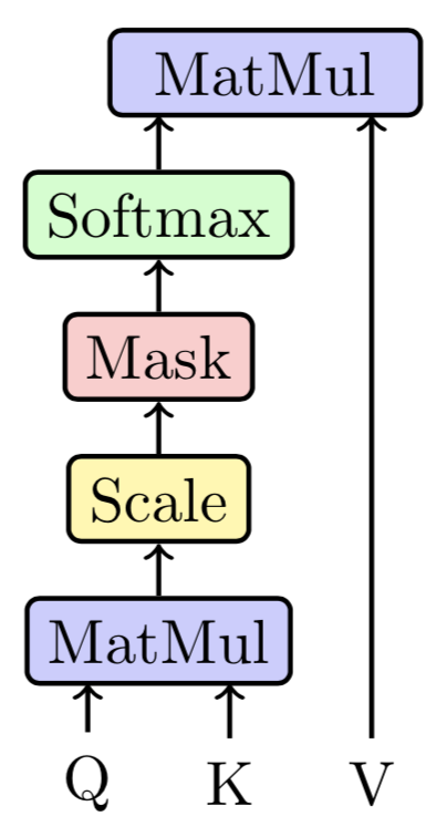
By the end of this tutorial, you should be able to recreate a basic diagram, like this single attention head.
1 | |
The TeX source for this post may be found here.
Basics
All TikZ pictures are drawn within a tikzpicture environment.
Within this environment, items are drawn onto an underlying Cartesian plane.
In this tutorial, I will refer to this plane as the document grid.
Many diagrams can be expressed as a graph,
with vertices connected by edges.
1 | |
We will refer to vertices as nodes
and the edges connecting them as paths.
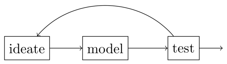
With this terminology, let us break down the construction of this drawing.
- There are three nodes in this drawing, corresponding to “ideate,” “model,” and “test.” Each node is placed within the document grid at a fixed position, which may be absolute or relative. Here, the nodes are placed at the absolute positions of $(0,0),(2,0),(4,0)$. We will discuss relative positioning at a later time.
- Each node is required to have a
label, which may be empty. The label is displayed in your drawing. Each node may also have aname, which is an internal reference for the node. While strictly optional, naming nodes is highly recommended so you can reference them later, whether to position other nodes or to draw paths between nodes. -
With that in mind, we can connect nodes. There are two ways to do this,
\drawand\path. These commands differ in subtle ways, and I personally find that the syntax for\pathis safer from beginner bugs.Paths are decently self-explanatory: you can draw an
edgebetween any two points (nodes or coordinates) in the document grid, where each edge is a standalone path. Unless otherwise specified, edges point toward the center of each node.Finally, observe that one of the edges curves around. Options
bend rightorbend leftallows you to bend edges around obstacles.
Styles
Now that we have the basics down, we can make our nodes and edges look a little less barebones. Each node and path can take a set of options that specify its style and position. In this section we’ll focus on style.
Nodes
In the previous drawing, you may have noticed these options
that I passed to the tikzpicture environment:
The draw option specifies that we should draw a stroke
along each node’s boundary.
You can disable this via draw=none
or simply by omitting the draw option.
Here are some other styles you can explore.
1 | |

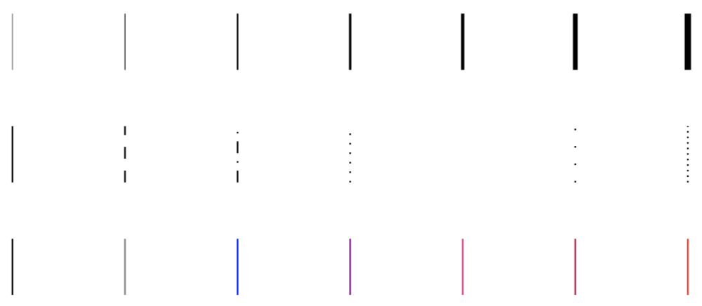
The thickness of your line is specified by
line width. This can be set to any numerical unit.
You may also use predefined thicknesses, which range from
ultra thin (far left) to ultra thick (far right).
The default line width is thin.
1 | |
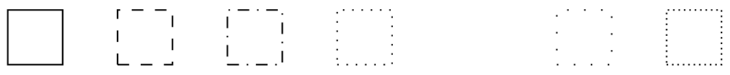
You can specify the dash pattern of each node.
There are three built-in variants:
dashed, dashdotted, and dotted.
These can be modified with loosely or densely.
1 | |

You can specify the color of each node’s stroke, fill, and label.
This reference
has a list of default colors, available in any system, as well as
colors available through the xcolor library.
While it’s possible to define your own colors,
it’s often easier to blend between existing colors with the syntax
color1 ! percentage color1 ! color2
If you do not specify a second color, the default is white.
1 | |
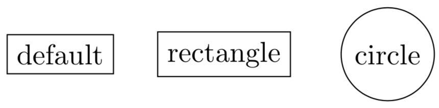
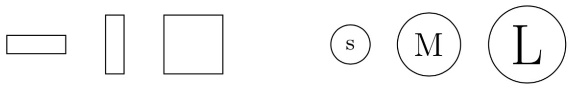
There are three built-in shapes:
rectangle, circle, and coordinate.
We can ignore coordinates for now.
By default, each node is a rectangle.
For more shapes you may load the shapes library.
1 | |
Finally, you might want to control the size of your nodes.
By default, nodes will always resize to fit their labels,
so vanilla TikZ only allows you to set the minimum size of a node.
However, you may tweak the inner sep of a node
to adjust the amount of padding between the text and the node boundary.
1 | |
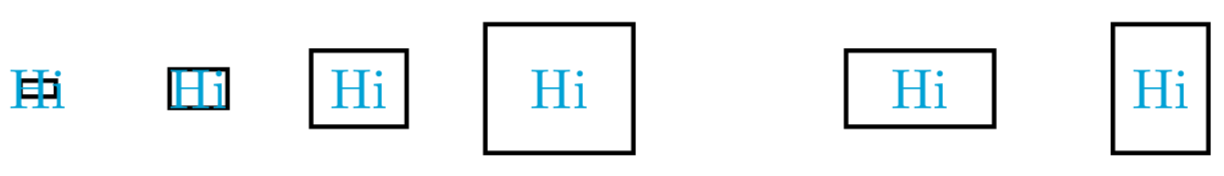
This padding may take on a negative value, and as usual, you can specify different x and y values.
Paths
Many of the styles that apply to nodes also apply to paths, including line width, dash pattern, and color.
1 | |
Now you might be thinking—the similarities end here, because paths can’t be circles—but actually, they can. To avoid confusion, however, we won’t discuss such paths in this tutorial. Instead, we’ll close off with some shapes that are relevant to paths: arrow tips.
1 | |
The general arrow tip syntax is start - end
where start and end may be empty.
The default arrow tip specified by > is the same as to,
similar to the math mode command, $\to$.
For more creative arrow tips, you may load the arrows library.
Conclusion
If you’ve followed up to here, you already have the ability to draw a wide range of diagrams—congrats!
At this point, I would recommend that you take out your $\LaTeX$ compiler and go draw some diagrams yourself. There will always be more syntax to be memorized, so there’s no hurry; now is the time to get your hands wet. Out into the TikZ world you go!
Acknowledgements
Thanks to Evan Chen and Tony Zhang for introducing me to $\LaTeX$ + TikZ when I was a baby freshman at MIT. Thanks to Yujia Bao for reading through my draft for this post.